Thursday, July 23, 2009

Volatility: The Black Hole of Leveraged ETFs

It seems that every day, new ETFs are being introduced in all different flavors. Growing more popular are leveraged and inverse ETFs, which are increasing in number at a rapid rate. Last week, I overheard two people on the train talking about the benefits of leveraged ETFs and how one can earn two or three times the market performance using these instruments. They concluded that investing in leveraged ETFs rather than their unlevered equivalents was a no brainer.

I quickly thought back to an article by Rodney Sullivan from the May/June issue of the CFA Institute Magazine that I had skimmed over the month before and decided that the merits of investing in leveraged ETFs would be a good topic for this forum.

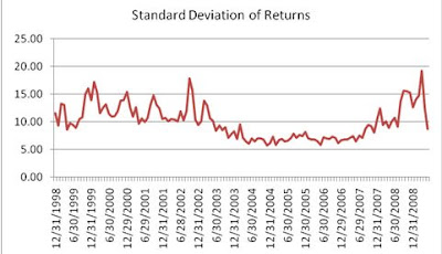
As we all know, volatility hurts our realized returns in the market. The higher the volatility of your daily or monthly returns, the more the geometric average return will deviate from the simple average return. For example, portfolio A, B, and C below all have identical average monthly returns (1%) over the 4 month period. You will earn the most money (4.06%) with A because it has the lowest volatility and the least money with portfolio C since it has the highest volatility. This is crucial to understanding the unforeseen impact volatility can have on the performance of leveraged ETFs.


Leveraged ETFs seek to return a multiple of the market return such as an Ultra 2X or 3X S&P 500 ETF. Over short time periods such as one day, the leveraged ETF will come very close to its goal. However, it only achieves the objective over that very short period. The YTD or one year performance of a leveraged ETF can be wildly different than expected.

In the example below, ETF A and ETF B trade once a month. Both investments earn 12.7% over the year such that a $100 investment in either one would yield $112.70 at the end of the year. ETF A earns that performance with a consistent monthly return of 1% and a standard deviation of 0%. ETF B, on the other hand, has high volatility with a standard deviation of 21%. Both ETFs have leveraged versions of two and three times the base return. One would think that since the annual performance of the base ETFs are equal, so should the annual performance of their leveraged equivalents.

The total one year returns of the leveraged versions of ETF A are roughly as expected at 2.1X and 3.4X the actual return for the year. However, for the high volatility ETF B, we get some alarming results for the leveraged versions. The 2X version returns -28.2% and the 3X version returns as seemingly impossible -85.7%. A $100 investment in the unleveraged ETF will become $112 at year-end while the same $100 investment in the leveraged 3X ETF will leave the investor with a measly $14 at year end.

The long term returns of leveraged ETFs are inherently unpredictable and can be significantly impacted by volatility. Multiplying the long-term performance of the base ETF by 2 or 3 does not produce an accurate estimate of the performance of the 2X and 3X ETFs over that same time period. Invest in these ultra ETFs with caution and understanding of the impact that volatility plays on performance.

Don't miss a post! Receive new blogs by e-mail.

Friday, July 17, 2009

HaR: Is your Holiday at Risk?

With the holiday season in front of us, I thought why not take a lighter perspective on the markets by asking, “Is your Holiday at Risk?” Concluding whether a holiday should be rescheduled might be taking it a step too far, but looking at the existence of seasonal patterns in the riskiness of equity markets is an interesting exercise. Therefore I decided to look at seasonality, first from a predicted /ex-ante and secondly from a realized/ex-post perspective.

Ex-Ante

I started off using a factor-based risk model to calculate a bottom up prediction of absolute risk (Total Risk in the lexicon of Barra Aegis). I looked at a broad market index, MSCI World Developed, over the last 10 years and used the Northfield Global Risk Model. One could see this as the predicted tracking error versus cash for the benchmark. I then averaged this data on a per-month basis across the years.


From the chart above we can observe the highest risk levels occur in and around January, and the lowest in and around October. Looking at a graph like this can be misleading, however, so I decided therefore to calculate a Welch’s T-test, and indeed none of the observations appeared significant. If we look at total risk levels over the last 10 years, it has varied quite a bit: from absolute highs around the tech bubble, to more moderate levels, and then back to higher levels more recently.


This led me to think that these differences in absolute levels might have some effects on the aggregated numbers. In order to control the variation in total risk levels, I also calculated the risk level relative to it’s three month trailing average.


This analysis confirms our earlier finding, that we find the lowest levels of risk around September, and the highs around the year end. Furthermore the Welch’s t test also confirmed that the risk is significantly different in September, December and January.

Ex-Post

In risk, one view is no view, therefore I also looked at risk from an ex-post or realized point of view. I wanted to look at measures that could be calculated on a monthly basis. I moved to Alpha Testing to analyze the cross sectional dispersion of returns. Again I focused on the MSCI World Developed over the last 10 years and first looked at the monthly standard deviation of returns.


We observe a similar pattern as for the predicted numbers, however it looks to be shifted a couple of months towards the beginning of the year. In other words we now find the lows in the summer rather than fall. I also looked at how the standard deviation developed over time. Again using the Welch’s T-test, it confirmed that the lower levels found in June to August are significantly different from the overall average.


Also, here we see some peaks around the tech bubble, and the more recent period. The differences seem less extreme compared to the predicted risk numbers. To get some more feel for the return distribution, I also reviewed the average kurtosis to see if we observe any fatter tails during specific months.


Looking at the chart, we observe a similar pattern. The highest kurtosis from February to April and relatively low kurtosis is seen from May to August. Furthermore, the lows in July and September and the high in December exhibited a statistically significant difference when compared to the other months.

Ex-Ante vs. Ex-Post

So, it looks like the ex-ante and ex-post measures tell a similar story but the ex-ante figures seem to lag somewhat. Therefore, I thought it interesting to also plot the predicted absolute risk and measure standard deviation of returns over time in one chart. The scales are obviously not directly comparable as they are different measures, but we would expect them to move consistently.


It seems difficult to draw any hard conclusions from this chart, although there are a couple of interesting things to notice. Both measures peak around the tech bubble and in the more recent periods. However for the standard devation we notice some extra oscillation after the tech bubble, and also the recent volatility seems to be picked up earlier.

Furthermore the standard deviation seems a lot more volatile than the predicted risk number. There’s some intuition to support that, it uses one month of data whereas the risk model used to calculate the predicted numbers uses 60 months (exponentially time-weighted, though).

Therefore one would expect to have somewhat smoothed results using the risk model. To put it differently, the risk models will need some time to reflect changing market conditions. Along the same lines, this can also explain why the ex-ante seasonal effect lags the ex-post findings. Perhaps moreso than the seasonality of risk, this outlines why one would need to think about using a shorter or longer horizon model.

Conclusions?

So what can we conclude from the above? There are two points that caught my attention. The first was already on my radar and again shouldn’t come as a surprise, risk levels have risen lately. However plotting and seeing the effect on actual numbers, I didn’t expect the differences to be so clear. Secondly it indeed looks like there is some seasonality in risk levels. Or perhaps I should phrase that more conservatively: a constant level of risk should never be assumed!


Stay up-to-date with our blog, receive new blog posts by e-mail.


This week's post was written by guest contributor Matthew van der Weide, Sales Specialist for Quantitative Services at FactSet's Benelux office.

Thursday, July 2, 2009

Everything seemed so much simpler back when we were young....

Following on from Chris Ellis' entry last week, I was intrigued enough by some of his risk measure selection expansions to go back to basics and consider some of the assumptions that we have come to completely accept, in particular, those of normality.

In Grinold & Kahn's Active Portfolio Management they use the distribution of the Magellan Fund's monthly returns and show that a normal assumption is a reasonable approximation for the distribution of these returns. From that we are taken through the use of standard deviation, variance, etc., and further into the use of tracking error at a portfolio level as a measure of active risk.

Using this as a starting point I took 60 months of returns of the Magellan Fund (I picked 60 as this is the standard period selected by most long term risk models) as of the data in the book ending on September 1994, and compared it with the same dataset generated as of the end of June 2009.


This is the 1994 data displayed graphically, and while we can see some negative skew to the chart and some small kurtosis around the mean, one can see how the normal distribution is a fair estimate for the distribution of the returns. As a check, we can go back to standard statistics when checking for the normality assumption, namely the mean, median, standard deviation, skew, and kurtosis.

The statistical table for the 1994 data vs. today's data is as follows:


There are several areas that I would like to highlight for you: the difference in mean return (a reflection of the cycle?); the spread between mean and median (highlighting skew); and most outstanding, the large difference in kurtosis, i.e., the existence of "fat tails"

In order to get a better understanding of the difference in values I plotted the frequency distribution chart for the last 60 months on the same scale as the 1994 one.


Again there looks to be a bias to the distribution, a skew, but what stands out immediately to me is that the outliers in the distribution are so much wider than they were and virtually beyond the limits of a normal assumption. Here the concept of fat tails can be easily seen and therefore more easily appreciated.

So I ask the question that I alluded to in the title of this blog, can the assumptions that used to serve us so well still be relied upon to continue to perform?

Please feel free to request the underlying data for the any of the above charts & tables.

Stay up-to-date with our blog, receive new blog posts by e-mail.